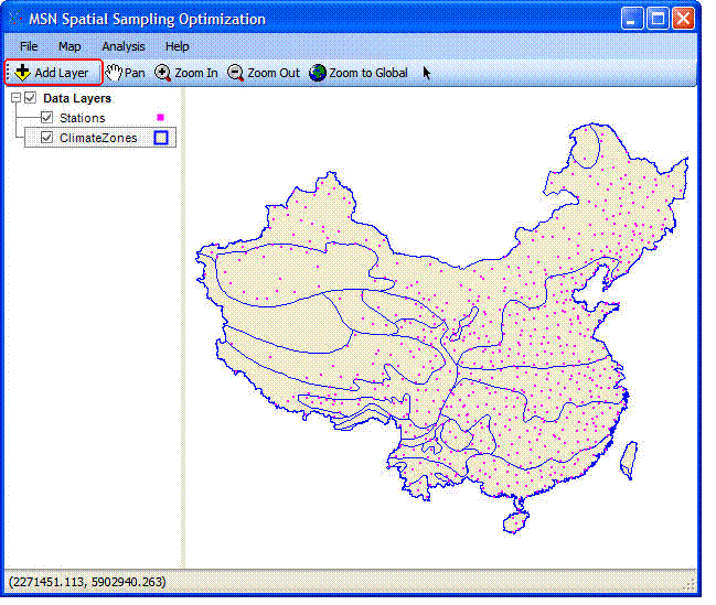
Case Study

The layout of the meteorological station was assessed based on the data of average temperatures between 1997 and 2007. There were mainly two steps: first of all, the average temperature and the estimated accuracy( averages and standard deviations) between 1997 and 2007 in our nation was estimated on the basis of the current site location and the monitoring data; What’s more, the specified estimated accuracy was set in order to improve the accuracy of estimation (reduce the estimated standard deviations); Finally, The station number required increasing was calculated and given a possible location of the distribution according to the given accuracy (Note: The unit of the temperature data: ℃)

Step 1: Load the meteorological station layer (Station.shp) and the climate zones layer (ClimateZones.shp)

Step 2: Begin the "Spatial Sampling Optimization Wizard" from the "Analysis" menu;

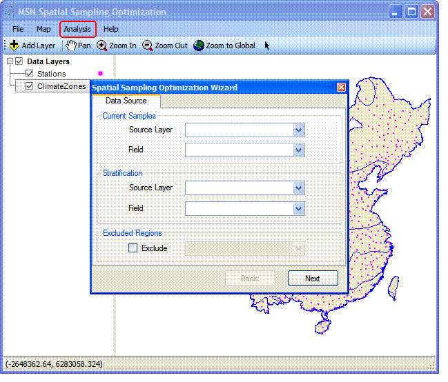
Note: “Excluded Regions” are regions that cannot put stations.

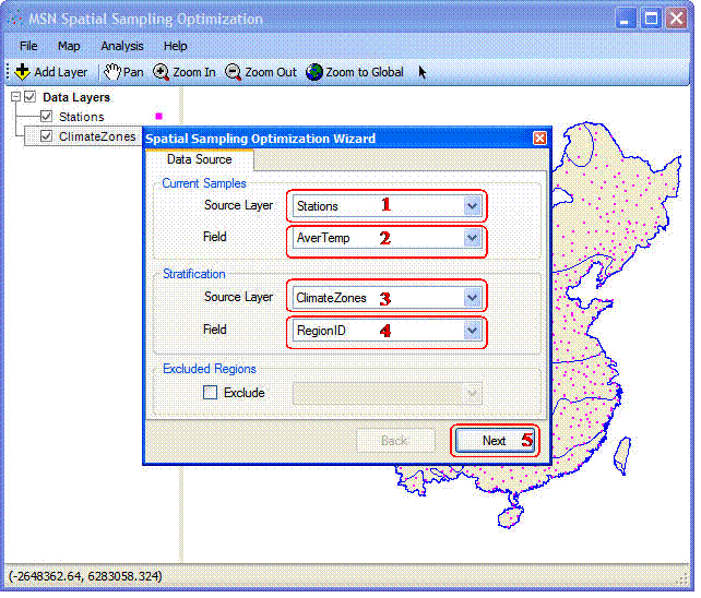
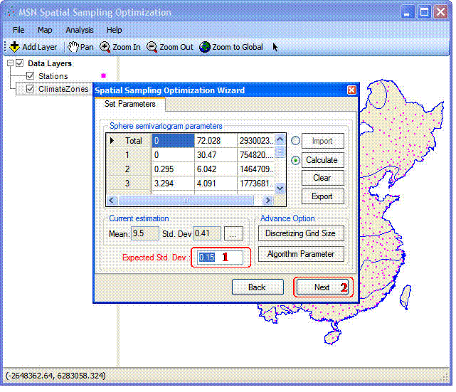
Step 3: In the "Data Source" page, select the relevant meteorological stations and climate partition information, and then click "Next."

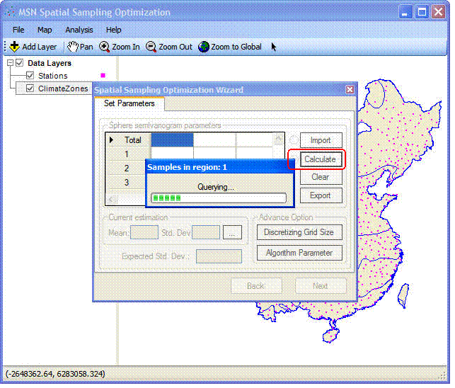
Step 4: In the "Set Parameters" page, three aspects of computing or settings are included:

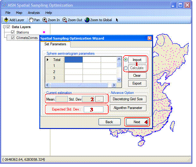
(1)  Calculate or Import “Sphere semi-variogram parameters”;

The results were as follows:

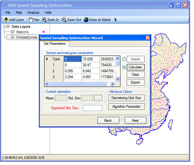
Note:

①The spherical model was used in this version of the software to descript the spatial relationship among the monitoring indexes. There were three parameters for each layer, namely, Nugget C0, partial sill C, and range a.

② The data in the grid’s first line were the global semi-variogram parameters of the investigation index (temperature); Other data from the second row until the last row were the semi-variogram parameters of each climatic zone.

③ If these parameters were imported from a text file by users, then the parameters of the whole and each climate zone accounted for a line, with comma separator.

④ It is important to note that the station number of each region should be at least greater than 5 if user chose to obtain the parameters in the methods of calculating; Otherwise, you will be prompted to take the global / overall parameters instead of the zone parameters.

⑤ The data in the grid can be modified by double-clicking the cells.

(2) After calculating/importing semi- variogram parameters, we can estimate the country's average temperature and the corresponding estimation standard deviation;

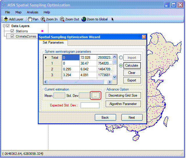
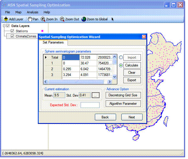
The results showed that the estimated average temperature was 9.5 ℃, and the standard deviation is about 0.41 ℃, under conditions of the present meteorological stations.

(3) In order to improve the estimated accuracy , for example the desired estimated accuracy is 0.15 ℃, the expected standard deviation is set as 0.15.

Click “next” to continue.

Note:

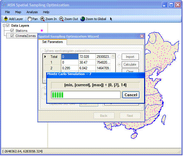
(1) The alternative sites were selected by the ways of Monte Carlo (MC) simulation first to reduce time. The minimum and maximum numbers were determined by last simulation.

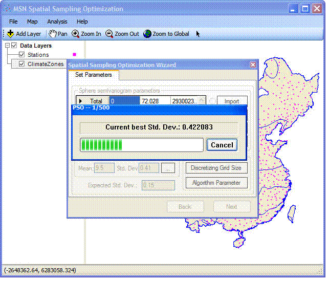
(2) If the MC simulation method cannot sites that meet the condition, it will resort to particle swarm optimization method to continue searching as following figure. Generally, this step is a little time consuming.

Step 5: Export calculation results.

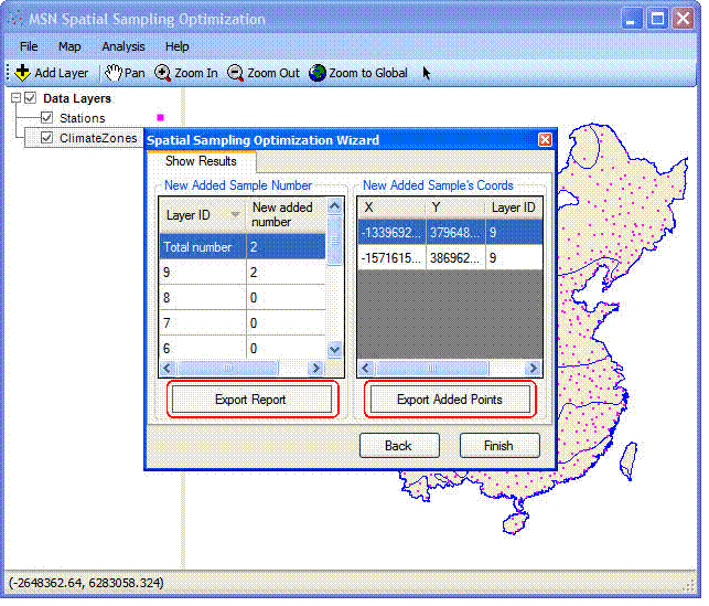
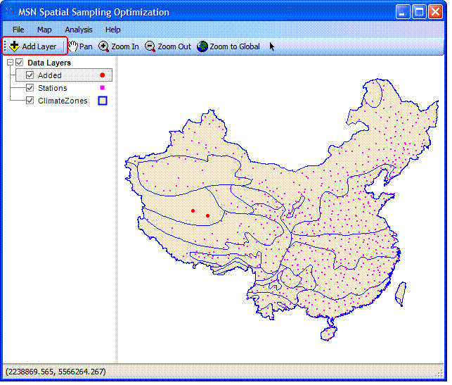
Step 6: View the new added site coordinates in the map.

About the "Advanced Options"

(1) Discrete Grid Size: The entire region is discretized to determine the population from which the added stations will be selected. The default population size is 3 times bigger than the current station number.

(2) Maximum simulation times: The new added meteorological stations are chosen from population by Monte Carlo simulations. The default simulation time is 500.